分享一下我老师大神的人工智能教程!零基础,通俗易懂!http://blog.csdn.net/jiangjunshow
也欢迎大家转载本篇文章。分享知识,造福人民,实现我们中华民族伟大复兴!
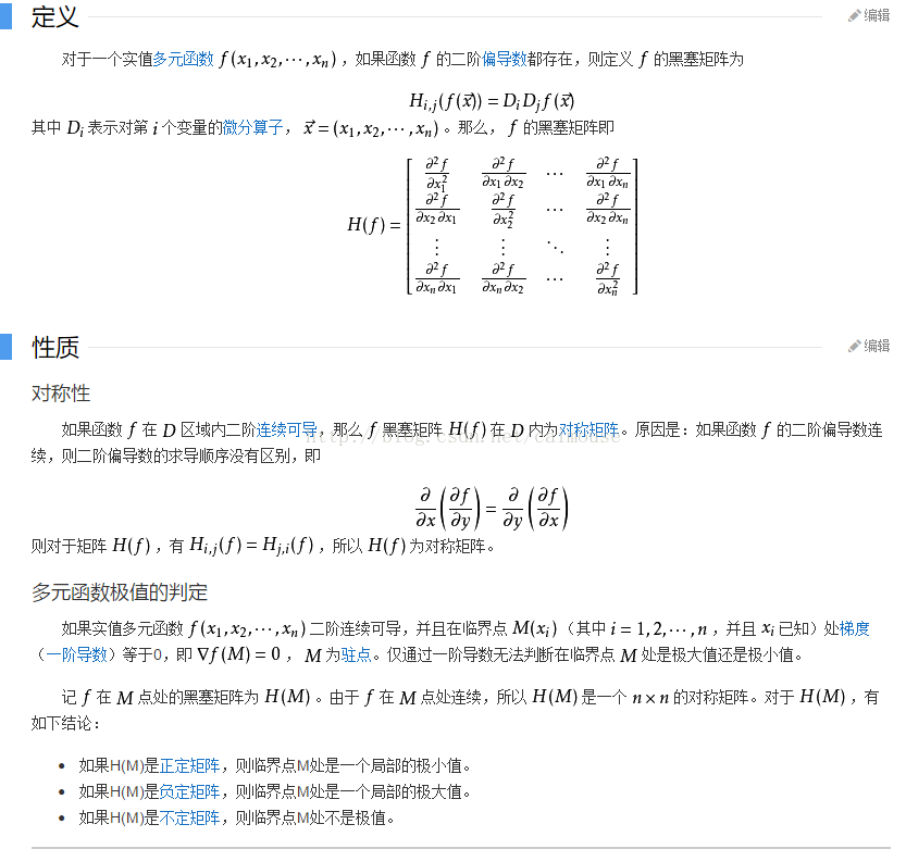
在机器学习课程里提到了这个矩阵,那么这个矩阵是从哪里来,又是用来作什么用呢?先来看一下定义:
黑塞矩阵(Hessian Matrix),又译作海森矩阵、海瑟矩阵、海塞矩阵等,是一个多元函数的二阶偏导数构成的方阵,描述了函数的局部曲率。黑塞矩阵最早于19世纪由德国数学家Ludwig Otto Hesse提出,并以其名字命名。黑塞矩阵常用于牛顿法解决优化问题。

一般来说, 牛顿法主要应用在两个方面, 1, 求方程的根; 2, 最优化.
在机器学习里,可以考虑采用它来计算n值比较少的数据,在图像处理里,可以抽取图像特征,在金融里可以用来作量化分析。
图像处理可以看这个连接:
http://blog.csdn.net/jia20003/article/details/16874237
量化分析可以看这个:
http://ookiddy.iteye.com/blog/2204127
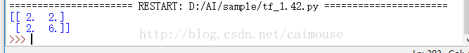
下面使用TensorFlow并且使用黑塞矩阵来求解下面的方程:

代码如下:
#python 3.5.3 蔡军生 #http://edu.csdn.net/course/detail/2592 # import tensorflow as tfimport numpy as npdef cons(x): return tf.constant(x, dtype=tf.float32)def compute_hessian(fn, vars): mat = [] for v1 in vars: temp = [] for v2 in vars: # computing derivative twice, first w.r.t v2 and then w.r.t v1 temp.append(tf.gradients(tf.gradients(f, v2)[0], v1)[0]) temp = [cons(0) if t == None else t for t in temp] # tensorflow returns None when there is no gradient, so we replace None with 0 temp = tf.stack(temp) mat.append(temp) mat = tf.stack(mat) return matx = tf.Variable(np.random.random_sample(), dtype=tf.float32)y = tf.Variable(np.random.random_sample(), dtype=tf.float32)f = tf.pow(x, cons(2)) + cons(2) * x * y + cons(3) * tf.pow(y, cons(2)) + cons(4)* x + cons(5) * y + cons(6)# arg1: our defined function, arg2: list of tf variables associated with the functionhessian = compute_hessian(f, [x, y])sess = tf.Session()sess.run(tf.global_variables_initializer())print(sess.run(hessian))输出结果如下:
再来举多一个例子的源码,它就是用来计算量化分析,这个代码很值钱啊,如下:
#python 3.5.3 蔡军生 #http://edu.csdn.net/course/detail/2592 # import numpy as npimport scipy.stats as statsimport scipy.optimize as opt#构造Hessian矩阵def rosen_hess(x): x = np.asarray(x) H = np.diag(-400*x[:-1],1) - np.diag(400*x[:-1],-1) diagonal = np.zeros_like(x) diagonal[0] = 1200*x[0]**2-400*x[1]+2 diagonal[-1] = 200 diagonal[1:-1] = 202 + 1200*x[1:-1]**2 - 400*x[2:] H = H + np.diag(diagonal) return Hdef rosen(x): """The Rosenbrock function""" return sum(100.0*(x[1:]-x[:-1]**2.0)**2.0 + (1-x[:-1])**2.0)def rosen_der(x): xm = x[1:-1] xm_m1 = x[:-2] xm_p1 = x[2:] der = np.zeros_like(x) der[1:-1] = 200*(xm-xm_m1**2) - 400*(xm_p1 - xm**2)*xm - 2*(1-xm) der[0] = -400*x[0]*(x[1]-x[0]**2) - 2*(1-x[0]) der[-1] = 200*(x[-1]-x[-2]**2) return derx_0 = np.array([0.5, 1.6, 1.1, 0.8, 1.2])res = opt.minimize(rosen, x_0, method='Newton-CG', jac=rosen_der, hess=rosen_hess, options={'xtol': 1e-8, 'disp': True})print("Result of minimizing Rosenbrock function via Newton-Conjugate-Gradient algorithm (Hessian):")print(res)输出结果如下:
====================== RESTART: D:/AI/sample/tf_1.43.py ======================
Optimization terminated successfully.
Current function value: 0.000000
Iterations: 20
Function evaluations: 22
Gradient evaluations: 41
Hessian evaluations: 20
Result of minimizing Rosenbrock function via Newton-Conjugate-Gradient algorithm (Hessian):
fun: 1.47606641102778e-19
jac: array([ -3.62847530e-11, 2.68148992e-09, 1.16637362e-08,
4.81693414e-08, -2.76999090e-08])
message: 'Optimization terminated successfully.'
nfev: 22
nhev: 20
nit: 20
njev: 41
status: 0
success: True
x: array([ 1., 1., 1., 1., 1.])
>>>
可见hessian矩阵可以使用在很多地方了吧。