在这篇机器学习入门教程中,我们将使用Python中最流行的机器学习工具scikit- learn,在Python中实现几种机器学习算法。使用简单的数据集来训练分类器区分不同类型的水果。

这篇文章的目的是识别出最适合当前问题的机器学习算法。因此,我们要比较不同的算法,选择性能最好的算法。让我们开始吧!
数据
水果数据集由爱丁堡大学的Iain Murray博士创建。他买了几十个不同种类的橘子、柠檬和苹果,并把它们的尺寸记录在一张桌子上。密歇根大学的教授们对水果数据进行了些微的格式化,可以从这里下载。
下载地址:https://github.com/susanli2016/Machine-Learning-with-Python/blob/master/fruit_data_with_colors.txt
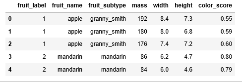
让我们先看一看数据的前几行。
import numpy as np
import pandas as pd
import matplotlib.pyplot as plt
fruits = pd.read_csv('fruit_data_with_colors.txt',sep='\t')
print(fruits.head())
数据集的每一行表示一个水果块,它由表中的几个特征表示。
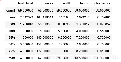
在数据集中有59个水果和7个特征:
print(fruits.shape)
(59, 7)
在数据集中有四种水果:
print(fruits['fruit_name'].unique())
[“苹果”柑橘”“橙子”“柠檬”]
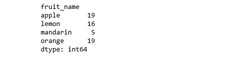
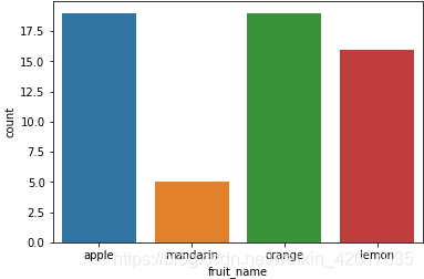
除了柑橘,数据是相当平衡的。我们只好接着进行下一步。
print(fruits.groupby('fruit_name').size())
import seaborn as sns
sns.countplot(fruits['fruit_name'],label="Count")
plt.show()
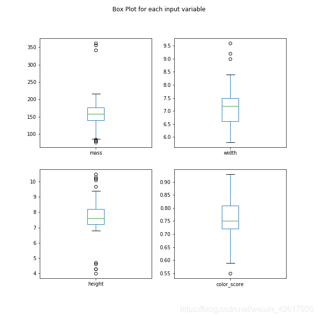
#每个数字变量的箱线图将使我们更清楚地了解输入变量的分布:
fruits.drop('fruit_label', axis=1).plot(kind='box', subplots=True, layout=(2,2), sharex=False, sharey=False, figsize=(9,9),
                                        title='Box Plot for each input variable')
plt.savefig('fruits_box')
plt.show()
看起来颜色分值近似于高斯分布。
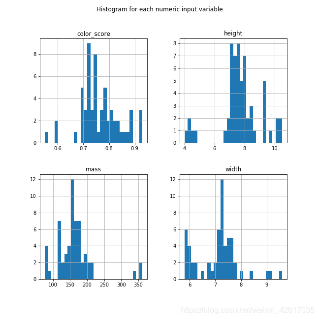
显示各属性的直方图
#显示各属性的直方图
import pylab as pl
fruits.drop('fruit_label' ,axis=1).hist(bins=30, figsize=(9,9))
pl.suptitle("Histogram for each numeric input variable")
plt.savefig('fruits_hist')
plt.show()
一些成对的属性是相关的(质量和宽度)。这表明了高度的相关性和可预测的关系。
#通过散点矩阵图查看属性之间的相关性
from pandas.plotting import scatter_matrix
from matplotlib import cm
feature_names = ['mass', 'width', 'height', 'color_score']
X = fruits[feature_names]
y = fruits['fruit_label']
cmap = cm.get_cmap('gnuplot')
scatter = scatter_matrix(X, c = y, marker = 'o', s=40, hist_kwds={'bins':15}, figsize=(9,9), cmap = cmap)
plt.suptitle('Scatter-matrix for each input variable')
plt.savefig('fruits_scatter_matrix')
plt.show()
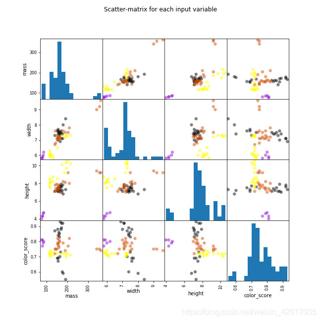
我们可以看到数值没有相同的缩放比例。我们需要将缩放比例扩展应用到我们为训练集计算的测试集上。
创建训练和测试集,并应用缩放比例
#创建训练和测试集,并应用缩放比例
from sklearn.model_selection import train_test_split
X_train, X_test, y_train, y_test = train_test_split(X, y, random_state=0)
from sklearn.preprocessing import MinMaxScaler
scaler = MinMaxScaler()
X_train = scaler.fit_transform(X_train)
X_test = scaler.transform(X_test)
构建模型
逻辑回归
#逻辑回归
from sklearn.linear_model import LogisticRegression
logreg = LogisticRegression()
logreg.fit(X_train, y_train)
print('Accuracy of Logistic regression classifier on training set: {:.2f}'
     .format(logreg.score(X_train, y_train)))
print('Accuracy of Logistic regression classifier on test set: {:.2f}'
     .format(logreg.score(X_test, y_test)))
训练集中逻辑回归分类器的精确度:0.70
测试集中逻辑回归分类器的精确度:0.40
决策树
#决策树
from sklearn.tree import DecisionTreeClassifier
clf = DecisionTreeClassifier().fit(X_train, y_train)
print('Accuracy of Decision Tree classifier on training set: {:.2f}'
     .format(clf.score(X_train, y_train)))
print('Accuracy of Decision Tree classifier on test set: {:.2f}'
     .format(clf.score(X_test, y_test)))
训练集中决策树分类器的精确度:1.00
测试集中决策树分类器的精确度:0.73
K-Nearest Neighbors(K-NN )
#K-Nearest Neighbors(K-NN)
from sklearn.neighbors import KNeighborsClassifier
knn = KNeighborsClassifier()
knn.fit(X_train, y_train)
print('Accuracy of K-NN classifier on training set: {:.2f}'
     .format(knn.score(X_train, y_train)))
print('Accuracy of K-NN classifier on test set: {:.2f}'
     .format(knn.score(X_test, y_test)))
训练集中K-NN 分类器的精确度:0.95
测试集中K-NN 分类器的精确度:1.00
线性判别分析
#线性判别分析
from sklearn.discriminant_analysis import LinearDiscriminantAnalysis
lda = LinearDiscriminantAnalysis()
lda.fit(X_train, y_train)
print('Accuracy of LDA classifier on training set: {:.2f}'
     .format(lda.score(X_train, y_train)))
print('Accuracy of LDA classifier on test set: {:.2f}'
     .format(lda.score(X_test, y_test)))
训练集中LDA分类器的精确度:0.86
测试集中LDA分类器的精确度:0.67
高斯朴素贝叶斯
#高斯朴素贝叶斯
from sklearn.naive_bayes import GaussianNB
gnb = GaussianNB()
gnb.fit(X_train, y_train)
print('Accuracy of GNB classifier on training set: {:.2f}'
     .format(gnb.score(X_train, y_train)))
print('Accuracy of GNB classifier on test set: {:.2f}'
     .format(gnb.score(X_test, y_test)))
训练集中GNB分类器的精确度:0.86
测试集中GNB分类器的精确度:0.67
支持向量机
#支持向量机
from sklearn.svm import SVC
svm = SVC()
svm.fit(X_train, y_train)
print('Accuracy of SVM classifier on training set: {:.2f}'
     .format(svm.score(X_train, y_train)))
print('Accuracy of SVM classifier on test set: {:.2f}'
     .format(svm.score(X_test, y_test)))
训练集中SVM分类器的精确度:0.61
测试集中SVM分类器的精确度:0.33
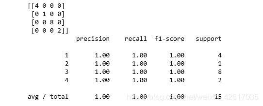
KNN算法是我们尝试过的最精确的模型。混淆矩阵提供了在测试集上没有错误的指示。但是,测试集非常小。
#KNN算法是我们尝试过的最精确的模型。混淆矩阵提供了在测试集上没有错误的指示。不过,测试集非常小。
from sklearn.metrics import classification_report
from sklearn.metrics import confusion_matrix
pred = knn.predict(X_test)
print(confusion_matrix(y_test, pred))
print(classification_report(y_test, pred))
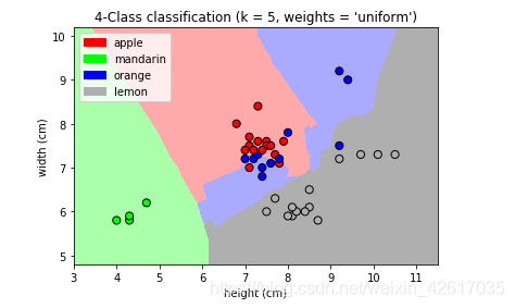
绘制k-NN分类器的决策边界
'''
绘制k-NN分类器的决策边界
'''
import matplotlib.cm as cm
from matplotlib.colors import ListedColormap, BoundaryNorm
import matplotlib.patches as mpatches
import matplotlib.patches as mpatches

X = fruits[['mass', 'width', 'height', 'color_score']]
y = fruits['fruit_label']
X_train, X_test, y_train, y_test = train_test_split(X, y, random_state=0)

def plot_fruit_knn(X, y, n_neighbors, weights):
    X_mat = X[['height', 'width']].values
    y_mat = y.values
    # Create color maps
    cmap_light = ListedColormap(['#FFAAAA', '#AAFFAA', '#AAAAFF', '#AFAFAF'])
    cmap_bold = ListedColormap(['#FF0000', '#00FF00', '#0000FF', '#AFAFAF'])

    clf = KNeighborsClassifier(n_neighbors, weights=weights)
    clf.fit(X_mat, y_mat)
    # Plot the decision boundary by assigning a color in the color map
    # to each mesh point.

    mesh_step_size = .01  # step size in the mesh
    plot_symbol_size = 50

    x_min, x_max = X_mat[:, 0].min() - 1, X_mat[:, 0].max() + 1
    y_min, y_max = X_mat[:, 1].min() - 1, X_mat[:, 1].max() + 1
    xx, yy = np.meshgrid(np.arange(x_min, x_max, mesh_step_size),
                         np.arange(y_min, y_max, mesh_step_size))
    Z = clf.predict(np.c_[xx.ravel(), yy.ravel()])
    # Put the result into a color plot
    Z = Z.reshape(xx.shape)
    plt.figure()
    plt.pcolormesh(xx, yy, Z, cmap=cmap_light)
    # Plot training points
    plt.scatter(X_mat[:, 0], X_mat[:, 1], s=plot_symbol_size, c=y, cmap=cmap_bold, edgecolor='black')
    plt.xlim(xx.min(), xx.max())
    plt.ylim(yy.min(), yy.max())
    patch0 = mpatches.Patch(color='#FF0000', label='apple')
    patch1 = mpatches.Patch(color='#00FF00', label='mandarin')
    patch2 = mpatches.Patch(color='#0000FF', label='orange')
    patch3 = mpatches.Patch(color='#AFAFAF', label='lemon')
    plt.legend(handles=[patch0, patch1, patch2, patch3])
    plt.xlabel('height (cm)')
    plt.ylabel('width (cm)')
    plt.title("4-Class classification (k = %i, weights = '%s')"
              % (n_neighbors, weights))
    plt.show()

plot_fruit_knn(X_train, y_train, 5, 'uniform')
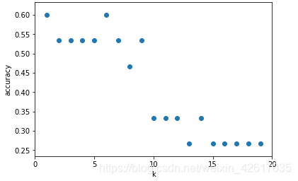
查找最优的k值
'''
查找最优的k值
'''
k_range = range(1, 20)
scores = []
#对于这个特定的数据集,当k为1、6时,我们获得了最高精确度。
for k in k_range:
    knn = KNeighborsClassifier(n_neighbors = k)
    knn.fit(X_train, y_train)
    scores.append(knn.score(X_test, y_test))
plt.figure()
plt.xlabel('k')
plt.ylabel('accuracy')
plt.scatter(k_range, scores)
plt.xticks([0,5,10,15,20])
plt.show()
对于这个特定的数据集,当k为1、6时,我们获得了最高精确度。
转载自原文链接, 如需删除请联系管理员。
原文链接:六种分类算法的比较——以水果分类为例,转载请注明来源!