Kaggle 竞赛项目——Rossmann 销售预测 Top1%

# coding: utf-8

#开发环境：windows10, Anacoda3.5 , jupyter notebook ,python3.6 
#库： numpy,pandas,matplotlib,seaborn,xgboost,time
#运行时间：CPU: i7-6700HQ，约8h

#项目名称： Rossmann 销售预测

# 1.数据分析

# In[1]:


#导入所需要的库
import numpy as np
import pandas as pd
import seaborn as sns
import matplotlib.pyplot as plt
get_ipython().run_line_magic('matplotlib', 'inline')
import xgboost as xgb
from time import time


# In[2]:


#读取数据
train = pd.read_csv('train.csv',parse_dates=[2])
test = pd.read_csv('test.csv',parse_dates=[3])
store = pd.read_csv('store.csv')


# In[3]:


#查看训练集
train.head().append(train.tail())


# In[4]:


#查看测试集
test.head().append(test.tail())


# In[5]:


#查看店铺信息
store.head().append(store.tail())


# In[6]:


#查看数据缺失
display(train.isnull().sum(),test.isnull().sum(),store.isnull().sum())


# In[7]:


#缺失数据分析
#测试集缺失数据
test[pd.isnull(test.Open)]


# - 缺失数据都来自于622店铺，从周1到周6而且没有假期，所以我们认为这个店铺的状态应该是正常营业的

# In[8]:


#店铺集缺失数据
store[pd.isnull(store.CompetitionDistance)]


# In[9]:


store[pd.isnull(store.CompetitionOpenSinceMonth)].head(10)


# In[10]:


#查看是否Promo2系列的缺失是否是因为没有参加促销
NoPW = store[pd.isnull(store.Promo2SinceWeek)]
NoPW[NoPW.Promo2 != 0].shape


# - 店铺竞争数据缺失的原因不明，且数量比较多，我们可以用中值或者0来填充，后续的实验发现以0填充的效果更好
# - 店铺促销信息的缺失是因为没有参加促销活动，所以我们以0填充

# In[11]:


#分析店铺销量随时间的变化
strain = train[train.Sales>0]
strain.loc[strain['Store']==1 ,['Date','Sales']]     .plot(x='Date',y='Sales',title='Store1',figsize=(16,4))


# In[12]:


#分析店铺6-9月份的销量变化
strain = train[train.Sales>0]
strain.loc[strain['Store']==1 ,['Date','Sales']]     .plot(x='Date',y='Sales',title='Store1',figsize=(8,2),xlim=['2014-6-1','2014-7-31'])
strain.loc[strain['Store']==1 ,['Date','Sales']]     .plot(x='Date',y='Sales',title='Store1',figsize=(8,2),xlim=['2014-8-1','2014-9-30'])


# - 从上图的分析中，我们可以看到店铺的销售额是有周期性变化的，一年之中11，12月份销量要高于其他月份，可能有季节因素或者促销等原因.
# - 此外从对2014年6月-9月份的销量来看，6，7月份的销售趋势与8，9月份类似，因为我们需要预测的6周在2015年8，9月份，因此我们可以把2015年6，7月份最近的6周数据作为hold-out数据集，用于模型的优化和验证。

# 2.数据预处理

# In[13]:


#缺失值处理
#我们将test中的open数据补为1，即营业状态
test.fillna(1, inplace=True)
#store['CompetitionDistance'].fillna(store['CompetitionDistance'].median(), inplace = True)
#store['CompetitionOpenScinceYear'].fillna(store['CompetitionDistance'].median(), inplace = True)
#store['CompetitionOPenScinceMonth'].fillna(store['CompetitionDistance'].median(), inplace = True)

#store中的缺失数据大多与竞争对手和促销有关，在实验中我们发现竞争对手信息的中值填充效果并不好，所以这里统一采用0填充
store.fillna(0, inplace=True)


# In[14]:


#查看是否还存在缺失值
display(train.isnull().sum(),test.isnull().sum(),store.isnull().sum())


# In[15]:


#合并store信息
train = pd.merge(train, store, on='Store')
test = pd.merge(test, store, on='Store')


# In[16]:


#留出最近的6周数据作为hold_out数据集进行测试
train = train.sort_values(['Date'],ascending = False)
ho_test = train[:6*7*1115]
ho_train = train[6*7*1115:]


# In[17]:


#因为销售额为0的记录不计入评分，所以只采用店铺为开，且销售额大于0的数据进行训练
ho_test = ho_test[ho_test["Open"] != 0]
ho_test = ho_test[ho_test["Sales"] > 0]
ho_train = ho_train[ho_train["Open"] != 0]
ho_train = ho_train[ho_train["Sales"] > 0]


# 3.特征工程

# In[18]:


#特征处理与转化，定义特征处理函数
def features_create(data):
    
    #将存在其他字符表示分类的特征转化为数字
    mappings = {'0':0, 'a':1, 'b':2, 'c':3, 'd':4}
    data.StoreType.replace(mappings, inplace=True)
    data.Assortment.replace(mappings, inplace=True)
    data.StateHoliday.replace(mappings, inplace=True)
    
    #将时间特征进行拆分和转化，并加入'WeekOfYear'特征
    data['Year'] = data.Date.dt.year
    data['Month'] = data.Date.dt.month
    data['Day'] = data.Date.dt.day
    data['DayOfWeek'] = data.Date.dt.dayofweek
    data['WeekOfYear'] = data.Date.dt.weekofyear
    
    
    #新增'CompetitionOpen'和'PromoOpen'特征,计算某天某店铺的竞争对手已营业时间和店铺已促销时间，用月为单位表示
    data['CompetitionOpen'] = 12 * (data.Year - data.CompetitionOpenSinceYear) +         (data.Month - data.CompetitionOpenSinceMonth)
    data['PromoOpen'] = 12 * (data.Year - data.Promo2SinceYear) +         (data.WeekOfYear - data.Promo2SinceWeek) / 4.0
    data['CompetitionOpen'] = data.CompetitionOpen.apply(lambda x: x if x > 0 else 0)        
    data['PromoOpen'] = data.PromoOpen.apply(lambda x: x if x > 0 else 0)
    
    
    #将'PromoInterval'特征转化为'IsPromoMonth'特征,表示某天某店铺是否处于促销月，1表示是，0表示否
    month2str = {1:'Jan', 2:'Feb', 3:'Mar', 4:'Apr', 5:'May', 6:'Jun',              7:'Jul', 8:'Aug', 9:'Sept', 10:'Oct', 11:'Nov', 12:'Dec'}
    data['monthStr'] = data.Month.map(month2str)
    data.loc[data.PromoInterval == 0, 'PromoInterval'] = ''
    data['IsPromoMonth'] = 0
    for interval in data.PromoInterval.unique():
        if interval != '':
            for month in interval.split(','):
                data.loc[(data.monthStr == month) & (data.PromoInterval == interval), 'IsPromoMonth'] = 1

    return data


# In[19]:


#对训练，保留以及测试数据集进行特征转化
features_create(ho_train)
features_create(ho_test)
features_create(test)
print('Features creation finished')


# In[20]:


#删掉训练和保留数据集中不需要的特征
ho_train.drop(['Date','Customers','Open','PromoInterval','monthStr'],axis=1,inplace =True)
ho_test.drop(['Date','Customers','Open','PromoInterval','monthStr'],axis=1,inplace =True)


# In[21]:


#分析训练数据集中特征相关性以及特征与'Sales'标签相关性
plt.subplots(figsize=(24,20))
sns.heatmap(ho_train.corr(),annot=True, vmin=-0.1, vmax=0.1,center=0)


# In[22]:


#拆分特征与标签，并将标签取对数处理
ho_xtrain = ho_train.drop(['Sales'],axis=1 )
ho_ytrain = np.log1p(ho_train.Sales)
ho_xtest = ho_test.drop(['Sales'],axis=1 )
ho_ytest = np.log1p(ho_test.Sales)


# In[23]:


#删掉测试集中对应的特征与训练集保持一致
xtest =test.drop(['Id','Date','Open','PromoInterval','monthStr'],axis = 1)


# 4.定义评价函数

# In[24]:


#定义评价函数rmspe
def rmspe(y, yhat):
    return np.sqrt(np.mean((yhat/y-1) ** 2))

def rmspe_xg(yhat, y):
    y = np.expm1(y.get_label())
    yhat = np.expm1(yhat)
    return "rmspe", rmspe(y,yhat)


# 5.模型构建

# In[25]:


#初始模型构建
#参数设定
params = {"objective": "reg:linear",
          "booster" : "gbtree",
          "eta": 0.03,
          "max_depth": 10,
          "subsample": 0.9,
          "colsample_bytree": 0.7,
          "silent": 1,
          "seed": 10
          }
num_boost_round = 6000


dtrain = xgb.DMatrix(ho_xtrain, ho_ytrain)
dvalid = xgb.DMatrix(ho_xtest, ho_ytest)
watchlist = [(dtrain, 'train'), (dvalid, 'eval')]

#模型训练
print("Train a XGBoost model")
start = time()
gbm = xgb.train(params, dtrain, num_boost_round, evals=watchlist, 
  early_stopping_rounds=100, feval=rmspe_xg, verbose_eval=True)
end = time()
print('Training time is {:2f} s.'.format(end-start))

#采用保留数据集进行检测
print("validating")
ho_xtest.sort_index(inplace=True) 
ho_ytest.sort_index(inplace=True) 
yhat = gbm.predict(xgb.DMatrix(ho_xtest))
error = rmspe(np.expm1(ho_ytest), np.expm1(yhat))

print('RMSPE: {:.6f}'.format(error))



# 6.结果分析

# In[26]:


#构建保留数据集预测结果
res = pd.DataFrame(data = ho_ytest)
res['Prediction']=yhat
res = pd.merge(ho_xtest,res, left_index= True, right_index=True)
res['Ratio'] = res.Prediction/res.Sales
res['Error'] =abs(res.Ratio-1)
res['Weight'] = res.Sales/res.Prediction
res.head()


# In[27]:


#分析保留数据集中任意三个店铺的预测结果
col_1 = ['Sales','Prediction']
col_2 = ['Ratio']
L=np.random.randint( low=1,high = 1115, size = 3 ) 
print('Mean Ratio of predition and real sales data is {}: store all'.format(res.Ratio.mean()))
for i in L:
    
    s1 = pd.DataFrame(res[res['Store']==i],columns = col_1)
    s2 = pd.DataFrame(res[res['Store']==i],columns = col_2)
    s1.plot(title = 'Comparation of predition and real sales data: store {}'.format(i),figsize=(12,4))
    s2.plot(title = 'Ratio of predition and real sales data: store {}'.format(i),figsize=(12,4))
    print('Mean Ratio of predition and real sales data is {}: store {}'.format(s2.Ratio.mean(),i))



# In[28]:


#分析偏差最大的10个预测结果
res.sort_values(['Error'],ascending=False,inplace= True)
res[:10]


# - 从分析结果来看，我们的初始模型已经可以比较好的预测hold-out数据集的销售趋势，但是相对真实值，我们的模型的预测值整体要偏高一些。从对偏差数据分析来看，偏差最大的3个数据也是明显偏高。因此我们可以以hold-out数据集为标准对模型进行偏差校正。

# 7.模型优化

# In[29]:


#7.1偏差整体校正优化
print("weight correction")
W=[(0.990+(i/1000)) for i in range(20)]
S =[]
for w in W:
    error = rmspe(np.expm1(ho_ytest), np.expm1(yhat*w))
    print('RMSPE for {:.3f}:{:.6f}'.format(w,error))
    S.append(error)
Score = pd.Series(S,index=W)
Score.plot()
BS = Score[Score.values == Score.values.min()]
print ('Best weight for Score:{}'.format(BS))


# - 当校正系数为0.995时，hold-out集的RMSPE得分最低：0.118889，相对于初始模型 0.125453得分有很大的提升。

# - 因为每个店铺都有自己的特点，而我们设计的模型对不同的店铺偏差并不完全相同，所以我们需要根据不同的店铺进行一个细致的校正。

# In[30]:


#7.2细致校正：以不同的店铺分组进行细致校正，每个店铺分别计算可以取得最佳RMSPE得分的校正系数
L=range(1115)
W_ho=[]
W_test=[]
for i in L:
    s1 = pd.DataFrame(res[res['Store']==i+1],columns = col_1)
    s2 = pd.DataFrame(xtest[xtest['Store']==i+1])
    W1=[(0.990+(i/1000)) for i in range(20)]
    S =[]
    for w in W1:
        error = rmspe(np.expm1(s1.Sales), np.expm1(s1.Prediction*w))
        S.append(error)
    Score = pd.Series(S,index=W1)
    BS = Score[Score.values == Score.values.min()]
    a=np.array(BS.index.values)
    b_ho=a.repeat(len(s1))
    b_test=a.repeat(len(s2))
    W_ho.extend(b_ho.tolist())
    W_test.extend(b_test.tolist())


# In[31]:


#计算校正后整体数据的RMSPE得分
yhat_new = yhat*W_ho
error = rmspe(np.expm1(ho_ytest), np.expm1(yhat_new))
print ('RMSPE for weight corretion {:6f}'.format(error))


# - 细致校正后的hold-out集的得分为0.112010，相对于整体校正的0.118889的得分又有不小的提高

# In[32]:


#用初始和校正后的模型对训练数据集进行预测
print("Make predictions on the test set")
dtest = xgb.DMatrix(xtest)
test_probs = gbm.predict(dtest)

#初始模型
result = pd.DataFrame({"Id": test['Id'], 'Sales': np.expm1(test_probs)})
result.to_csv("Rossmann_submission_1.csv", index=False)

#整体校正模型
result = pd.DataFrame({"Id": test['Id'], 'Sales': np.expm1(test_probs*0.995)})
result.to_csv("Rossmann_submission_2.csv", index=False)

#细致校正模型
result = pd.DataFrame({"Id": test['Id'], 'Sales': np.expm1(test_probs*W_test)})
result.to_csv("Rossmann_submission_3.csv", index=False)


# - 然后我们用不同的seed训练10个模型,每个模型单独进行细致偏差校正后进行融合.

# In[33]:


#7.2训练融合模型
print("Train an new ensemble XGBoost model")
start = time()
rounds = 10
preds_ho = np.zeros((len(ho_xtest.index), rounds))
preds_test = np.zeros((len(test.index), rounds))
B=[]
for r in range(rounds):
    print('round {}:'.format(r+1))
    
    params = {"objective": "reg:linear",
          "booster" : "gbtree",
          "eta": 0.03,
          "max_depth": 10,
          "subsample": 0.9,
          "colsample_bytree": 0.7,
          "silent": 1,
          "seed": r+1
          }
    num_boost_round = 6000
    gbm = xgb.train(params, dtrain, num_boost_round, evals=watchlist, 
                    early_stopping_rounds=100, feval=rmspe_xg, verbose_eval=True)
    
    yhat = gbm.predict(xgb.DMatrix(ho_xtest))
    
    L=range(1115)
    W_ho=[]
    W_test=[]
    for i in L:
        s1 = pd.DataFrame(res[res['Store']==i+1],columns = col_1)
        s2 = pd.DataFrame(xtest[xtest['Store']==i+1])
        W1=[(0.990+(i/1000)) for i in range(20)]
        S =[]
        for w in W1:
            error = rmspe(np.expm1(s1.Sales), np.expm1(s1.Prediction*w))
            S.append(error)
        Score = pd.Series(S,index=W1)
        BS = Score[Score.values == Score.values.min()]
        a=np.array(BS.index.values)
        b_ho=a.repeat(len(s1))
        b_test=a.repeat(len(s2))
        W_ho.extend(b_ho.tolist())
        W_test.extend(b_test.tolist())
    

    yhat_ho = yhat*W_ho
    yhat_test =gbm.predict(xgb.DMatrix(xtest))*W_test
    error = rmspe(np.expm1(ho_ytest), np.expm1(yhat_ho))
    B.append(error)
    preds_ho[:, r] = yhat_ho
    preds_test[:, r] = yhat_test
    print('round {} end'.format(r+1))
    
end = time()
time_elapsed = end-start
print('Training is end')
print('Training time is {} h.'.format(time_elapsed/3600))   



# In[34]:


#分析不同模型的相关性
preds = pd.DataFrame(preds_ho)
sns.pairplot(preds)


# - 模型融合可以采用简单平均或者加权重的方法进行融合。从上图来看，这10个模型相关性很高，差别不大，所以权重融合我们只考虑训练中单独模型在hold-out模型中的得分情况分配权重。

# In[35]:


#模型融合在hold-out数据集上的表现

#简单平均融合
print ('Validating')

bagged_ho_preds1 = preds_ho.mean(axis = 1)
error1 = rmspe(np.expm1(ho_ytest), np.expm1(bagged_ho_preds1))
print('RMSPE for mean: {:.6f}'.format(error1))

#加权融合
R = range(10)   
Mw = [0.20,0.20,0.10,0.10,0.10,0.10,0.10,0.10,0.00,0.00] 
A = pd.DataFrame()
A['round']=R
A['best_score']=B
A.sort_values(['best_score'],inplace = True)
A['weight']=Mw
A.sort_values(['round'],inplace = True)
weight=np.array(A['weight'])
preds_ho_w=weight*preds_ho
bagged_ho_preds2 = preds_ho_w.sum(axis = 1)
error2 = rmspe(np.expm1(ho_ytest), np.expm1(bagged_ho_preds2))
print('RMSPE for weight: {:.6f}'.format(error2))


# - 权重模型较均值模型有比较好的得分

# In[36]:


##用均值融合和加权融合后的模型对训练数据集进行预测
#均值融合
print("Make predictions on the test set")
bagged_preds = preds_test.mean(axis = 1)
result = pd.DataFrame({"Id": test['Id'], 'Sales': np.expm1(bagged_preds)})
result.to_csv("Rossmann_submission_4.csv", index=False)
#加权融合
bagged_preds = (preds_test*weight).sum(axis = 1)
result = pd.DataFrame({"Id": test['Id'], 'Sales': np.expm1(bagged_preds)})
result.to_csv("Rossmann_submission_5.csv", index=False)


# 8.模型特征重要性及最佳模型结果分析

# In[37]:


#模型特征重要性
xgb.plot_importance(gbm)


# - 从模型特征重要性分析，比较重要的特征有四类包括1.周期性特征'Day'，'DayOfWeek'，'WeekOfYera'，'Month'等，可见店铺的销售额与时间是息息相关的，尤其是周期较短的时间特征；2.店铺差异'Store'和'StoreTyp'特征，不同店铺的销售额存在特异性；3.短期促销（Promo)情况:'PromoOpen'和'Promo'特征，促销时间的长短与营业额相关性比较大；4.竞争对手相关特征包括：'CompetitionOpen'，‘CompetitionDistance'，'CompetitionOpenSinceMoth'以及'CompetitionOpenScinceyear'，竞争者的距离与营业年限对销售额有影响。
# - 作用不大的特征主要两类包括：1.假期特征：'SchoolHoliday'和'StateHoliday'，假期对销售额影响不大，有可能是假期店铺大多不营业，对模型预测没有太大帮助。2.持续促销(Promo2)相关的特征：'Promo2'，'Prom2SinceYear'以及'Prom2SinceWeek'等特征，有可能持续的促销活动对短期的销售额影响有限。

# In[38]:


#采用新的权值融合模型构建保留数据集预测结果
res1 = pd.DataFrame(data = ho_ytest)
res1['Prediction']=bagged_ho_preds2
res1 = pd.merge(ho_xtest,res1, left_index= True, right_index=True)
res1['Ratio'] = res1.Prediction/res.Sales
res1['Error'] =abs(res1.Ratio-1)
res1.head()


# In[39]:


#分析偏差最大的10个预测结果与初始模型差异
res1.sort_values(['Error'],ascending=False,inplace= True)
res['Store_new'] = res1['Store']
res['Error_new'] = res1['Error']
res['Ratio_new'] = res1['Ratio']
col_3 = ['Store','Ratio','Error','Store_new','Ratio_new','Error_new']
com = pd.DataFrame(res,columns = col_3)
com[:10]


# - 从新旧模型预测结果最大的几个偏差对比的情况来看，最终的融合模型在这几个预测值上大多有所提升，证明模型的校正和融合确实有效。

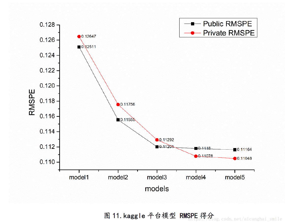
最佳模型kaggle prviate榜得分0.11048，排名20th

转载自原文链接, 如需删除请联系管理员。

原文链接：Kaggle 竞赛项目——Rossmann 销售预测 Top1%，转载请注明来源！