利用sklean的svm模块我们可以很容易做到分类:
x_train,x_test,y_train,y_test=model_selection.train_test_split(x,y,random_state=1,test_size=0.3)
classifier=svm.SVC(kernel='linear',gamma=0.8,decision_function_shape='ovo',C=1)
# kernel='rbf'(default)时,为高斯核函数
# kernel='linear'时,为线性核函数
classifier.fit(x_train,y_train)
最近遇到一个需求,三维特征分类后需要在三维图里画出超平面,网上搜了搜,
发现有个画二维的超平面的:
https://blog.csdn.net/qq_33039859/article/details/69810788
(此段代码来自这位作者的博客),感谢这位作者!
# get the separating hyperplane
w = clf.coef_[0]
a = -w[0] / w[1]
xx = np.linspace(-5, 5)
yy = a * xx - (clf.intercept_[0]) / w[1]

# plot the parallels to the separating hyperplane that pass through the
# support vectors
b = clf.support_vectors_[0]
yy_down = a * xx + (b[1] - a * b[0])
b = clf.support_vectors_[-1]
yy_up = a * xx + (b[1] - a * b[0])
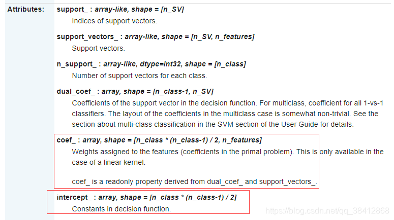
在文档里查到sklearn.svm.SVC分类器的属性:

至此还是没有太明白怎么计算超平面方程,接着在知乎上看到一位答主的例子,我恍然大悟:
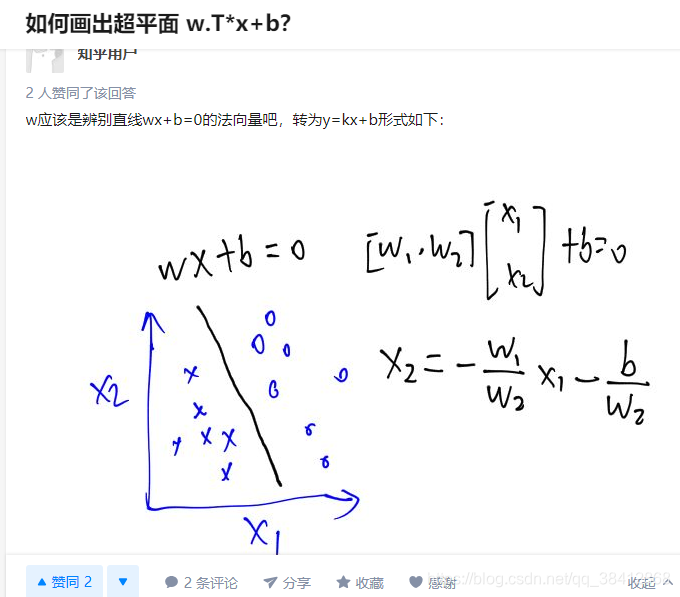
原来是这么算出来的,调包多了,果然菜的一笔
b=classifier.intercept_
w=classifier.coef_
通过intercept_属性可以得到shape = [n_class * (n_class-1) / 2, n_features]的矩阵(核函数为linear时才能用)
通过coef_属性可以得到shape = [n_class * (n_class-1) / 2]的矩阵
w的每一行对应于一个分类超平面的系数,b的每个对应于一个分类超平面的常数
即wx+b=0中的w和b
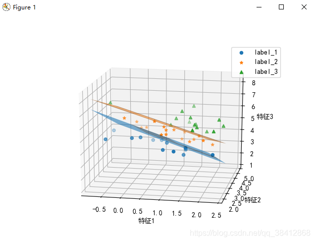
拿此次我的例子举例:
[w1,w2,w3][x1,x2,x3].T+b=0
可以解出x2=-w1/w3*x1-w2/w3*x2-b/w3
python代码:
#计算超平面方程wx+b=0
b=classifier.intercept_
w=classifier.coef_
xx = np.arange(min(x1),max(x1),1)
yy = np.arange(min(y1),max(y1),1)
X, Y = np.meshgrid(xx, yy)
Z1= -w[0,0]/w[0,2]*X-w[0,1]/w[0,2]*Y-b[0]/w[0,2]
Z2 = -w[1,0]/w[1,2]*X-w[1,1]/w[1,2]*Y-b[1]/w[1,2]
Z3 = -w[2,0]/w[2,2]*X-w[2,1]/w[2,2]*Y-b[2]/w[2,2]
#绘图
#设置默认字体
mpl.rcParams['font.sans-serif'] = [u'SimHei']
mpl.rcParams['axes.unicode_minus'] = False
fig = plt.figure()
ax = fig.add_subplot(111, projection='3d')
#画散点图
ax.scatter(x11,y11,z11,'r',marker='o',label='label_1')
ax.scatter(x22,y22,z22,'g',marker='*',label='label_2')
ax.scatter(x33,y33,z33,'b',marker='^',label='label_3')
#绘制超平面,alpha为设置平面透明度
ax.plot_surface(X,Y,Z1,alpha=0.6)
# ax.plot_surface(X,Y,Z2,alpha=0.6,)
ax.plot_surface(X,Y,Z3,alpha=0.6)
#设置轴标签
ax.set_xlabel("特征1",fontsize=10)
ax.set_ylabel("特征2",fontsize=10)
ax.set_zlabel("特征3",fontsize=10)
#设置图例
ax.legend(loc='best')
#保存图片
plt.savefig("Result.png")
plt.show()

转载自原文链接, 如需删除请联系管理员。
原文链接:利用sklearn.svm分类后如何画出超平面,转载请注明来源!